Extreme Cleverness: Functional Data Structures in Scala

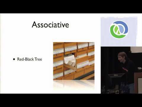
so uh in the Star Wars taxonomy of jvm language enthusiasts our next speaker uh corresponds to the young Anakin Skywalker his heart is in the right place but he is constantly seduced by the dark side I also believe that the inhuman amount of energy he displays when speaking is surely an indication that he has already begun the transformation to a cyborg and if you thought the last talk was too d for 9:00 in the morning well you ain't seen nothing yet so here we have Daniel spiwak to talk about functional data structures wow uh I am not sure I deserved any of that Stuart um okay functional data structures in Scola now the slide says in Scala um but the truth is that the majority of what I'm going to present here is is generic okay I'm going to be talking about different functional data structures and um kind of the concepts and ideas behind how they're implemented and there will be Scala on the screen but Don't Panic it's uh not really that complicated and um the majority of this is just going to be conceptual on High level so hopefully it's interesting and if not you can Stone me later um if you don't know what a functional data structure is you're probably in the wrong conference but we're going to cover what they are anyway just in case um but the main body of this talk is going to be um the kind of the theory and implementation of five different functional data structures Loosely categorized as sequential and associative now a sequential data structure is one that preserves insertion order and uh usually provides very fast access to either the head or the tail or maybe both but not so fast access to the stuff that's in the middle so Random Access not so good associative data structures are kind of orthogonal to this they don't preserve insertion order so it doesn't even make sense to ask about a head or a tail but what they provide is very consistent Random Access very consistently timed access to anything in the data structure and uh once we've looked at these implementations we're going to take a brief moment to look at some of the aspects of modern computer architecture that affect how we have to design data structures in a way that the theory just does not reflect U because there are some very surprising things that come from the fact that our code has to run on real machines and we can't just do it all in a whiteboard so what is a functional data structure well a functional data structure like almost everything in functional programming is one that is immutable okay it's an immutable data structure now these are actually very easy to write okay we could all write a functional array by just saying that every time you modify this array you make a copy of it and then you make the modification in the copy now this is great because it satisfies the definition of immutability but it is pathologically slow it's just ridiculous if you do this and uh it it really it's not as good as we could do if we were doing it in a mutable sense and this basically violates the first of our goals which is comparable ASM totic performance with our mutable counterparts Java util array list has a constant time modification operation to any element in the array and a constant time of pen so we want to be able to achieve that in a functional setting all right obviously this is going to be really hard to do but we want to try right and uh if we're just doing copy on right that's not constant time that's linear time so this is this is not so good and uh we want to do better than this but if we're doing an immutable data structure where we're not getting linear Time Performance then clearly we can't be touching every element in the data structure therefore some of it must be shared between the old version and the new version and this is this is what leads us to the idea of structural sharing which we're going to be looking at a lot this is the main tool this is the main trick that we're going to use to try to make these data structures better than just linear time all over the place so the first data structures we're going to look at are the sequential data structures and specifically the singly linked list now we're all familiar with this because it's really the canonical functional data structure and lisp is built on it but we're going to look at it anyway because it teaches us some important lessons so the complexity bounds for this data structure are somewhat unimpressive uh we can get at the head of the data structure in constant time but essentially anything else we might want to do with it is going to be linear time which is a little annoying but in practice you can make a lot of things work with it the nice thing about it is it's very simple to implement if you have a list it is one of two things it is either a conell with a head and a tail or it is the empty list and that's all you have to worry about so now in functional languages um most functional languages anyway when we want to implement a data structure the way we do it is we look at the cases that represent this data structure and then we Implement those cases as an algebraic data type and in Scala algebraic data types are represented by sealed traits and case classes so we've got our list trait here and then it's got two cases underneath it the cons case uh represented by the double colon since Scola likes ML and uh nil okay cons and nil cons has the head and the tail nail has nothing in it and we can Implement a cons method that takes an element and prepends it to the list and it's very very simple and this is all there is to it okay this is all there is to the list so um as I said the implementation is not interesting we're not learning anything here this is this is completely trivial what we are learning is something about structural sharing so let's say we had a list Fu that had four elements in it a b c and d we could represent it graphically like so now let's say we had another list bar that took H and prepended it to the taale of Fu if we represent this graphically um we could represent it by just another string of four nodes sort of uh H B C D nil sort of parallel to the one that we have for food but if we look at what this is in memory it's a little bit different H is prepended to the b c and d that are in f o fu that are in Fu so BC and D in Fu are shared between Fu and bar we could do this again with another data structure bass and we take M andn and prepend them to Foo itself and once again the elements that haven't changed are shared between versions of the data structure now we could make copies of these right we could copy b c and d we could copy a that would be fine it would be correct but really why bother a b c and d they're all immutable so what one copy is just as good as another we can share them we don't have to worry about different versions of the data structure stepping at each other we could do this again with a fourth data structure but I think you're kind of getting the idea here right we're sharing the pieces of the data structure that haven't change between subsequent versions now what we're seeing here is especially with things like bass prepended to Foo where all of fu is being shared with subsequent versions this is a very special property of the linked list okay you cannot do another data structure that shares everything every single time with every version of the data structure other structures are going to have to copy some things but our goal in every single case is to minimize the amount of copying and maximize the amount of sharing and when we can do that we can achieve very very powerful abstractions very very powerful functional data structures that are still immutable and maintain these nice guarantees so bankers Q okay well what is Banker Q well Banker's Q comes from a motivation for a functional Q we want a functional first in first out data structure and the most obvious thing to do here is to use the linked list right it's a nice sequential data structure very easy to implement in a functional context but it has a problem in that you uh you insert at one end okay and you could insert three elements a b c and d or a B and C AB C and D would be four elements which would be confusing and um if you remove from the head then you're going to get those three elements back C B A and that's not first in first out that is last in first out so it's not a q it's a stack we want a q so we would have to insert at the head of our list and remove from the tail but the problem is that inserting at the head is constant removing at the tail is linear and we could flip it around and insert it the tail and from the head but again one is going to be constant the other is going to be linear time and this violates our goal of comparable ASM totic performance because we have this nice Q data structure in mutable context that gives us constant time insert and remove so Banker Q is an attempt to do this and its complexity bounds are very very similar to the linked list uh with the exception of the fact that we have access to the the end of the structure we have the access to the end of the Q in constant time mostly um this we're going to talk about what amortization means but basically you should think of it as as this last operation is not quite as constant time as the other ones it's little bit less little bit less genuine so what is Banker's Q well Banker's Q is a naive persistent Q if you take the definition of functional persistence and the definition of a first in first out data structure mash them together in the dumbest way possible you will get Banker's queue it's it's really really straightforward you do it by taking two length lists two singly length lists one for the front one for the rear okay and for the front list you're going to use that for deqing you're going to remove elements from the front list and you're going to insert elements into the rear list now by itself this is a really bad strategy because the front list is just going to empty out and the rear list is just going to fill up and you're kind of in trouble so what you do is every time the front list gets to be smaller than the rear list you take the rear list reverse it and concatenate it onto the front list now of course this is a very expensive operation but you're not doing it all that often and this intuition is where we get to the argument about amortization so whenever you want to claim amortization you have to make the following argument most of the time when you perform an operation it is legitimately fast most of the time when we DQ when we remove something from that front list it is legitimately constant time removing the head of the list that's constant time with no tricks at all some of the time though we have to do something that's a little bit more expensive some of the time we have to do this whole reverse and concatenate Jazz and the argument we have to make is that the seldom run slow operation okay the reverse and concatenate thing is exponentially infrequent with respect to the fast operation and if you can make that argument then you can take the slow operation the cost of the slow operation and sort of distribute it over the cost of the fast operation and it all goes to a constant Factor over time right amortization and the neat thing about laziness if you do this with lazy singly link lists is it's literally taking this amortization idea this distribution of the cost and reifying it into the runtime so you're this whole reverse and concatenate thing if you have a lazy singly link list you can do that in constant time because all you have to do is create a function that will do it for you and you do have to pay the penalty eventually but you pay it as you are removing from that front list so you're Distributing the cost over all of the operations and you get a much more real time guarantee that way so what does this look like in code well our data structure is going to have as I promised two lazy signal length lists in Scola these are represented by stream and we're going to separately maintain the size of these lists so we can get at those sizes in constant time and our NQ and DQ operations are just going to operate on these lists in exactly the natural way possible take the result and run it through a check function and the check function takes a banker's queue and it looks at that Banker's queue and it asks itself is the front list still larger than the rear list if so then we're set right we don't have to do anything however if the front list has gotten to be smaller than the rear list then we take the rear list reverse it and concatenate it onto the front list return the new Bankers queue and reset so every time we perform an operation on Banker's queue we return the new Banker's queue and run it through the check function and that gives us that maintains our invariant so with this the NQ and DQ operations are very very very simple to implement we just operate on the front list or the rear list whatever it whatever operation we happen to be doing then run the result through the check function and we're done very very very very straightforward and surprisingly fast in practice this is a very very fast data structure when you actually run it but it's a bit of a hack okay we didn't really invent a new data structure here we didn't do anything particularly clever this is just a mashup of a data structure that we already had it would be nice if there were a data structure that were designed from the ground up to be a good functional CU and that data structure is the two three finger tree now the two three finger tree is about as complicated as it looks but it provides really really nice complexity guarantees okay basically we can get at either the head or the tail in constant time we can append we can prepend first or last and even things that we want to do in the middle of the data structure are probably going to be logarithmic time so this is pretty awesome in fact the two three finger tree is just about the IDE ideal sequential data structure it's pretty awesome it is the ideal persistent deck it is the ideal persistent double-ended Q basically if you take the definition of a double-ended q and uh the definition of persistence match them together and do the smartest most complicated thing possible you're going to get this um so how do we do this well what is our motivation well we want constant time access to both The Head and the tail so let's just take those elements and we're going to pull them up to the root okay we'll attach those elements to the root so that as long as we have the root of the tree we can always get at those elements in constant time and uh the the rest of the tree is going to be you know a sub tree inside of that right we'll just descend recursively and reset and this works great if all you're doing is reading right you're at the root you can read the the head or the tail in constant time super super simple the problem is if you are modifying this so what happens if you want to remove the head well we go down we pull out the head we remove that that's constant time but now we have this hole here so we have to replace that element so we walk down into the body remove its head pull it up now we have to replace that one so we're down and down and down and before you know it you're no longer constant time you're linear time because you have to descend halfway down the data structure half of the data structure has to be traversed so we have to do something about this and the trick we use is rather than just pulling up one element for the head and the tail one element for the prefix and the suffix we're going to pull up either two or three elements and we'll give ourselves fudge factors to four and one we'll let it sort of slide around but we're shooting for two or three and the argument kind of goes like this if you want to remove the head half of the time you are going to have three elements at the head so you remove one of them now you're down to two but that's okay two is all right and so you're set you just remove the head in constant time now the other half of the time you have to you're at two you remove one now you have to find some Replacements so you walk down into the body and you do the procedure again but half of the time you're going to be able to do that in the body in constant time the other half the time you descend down so half the time you're at the root a quarter of the time you're in the body an eighth of the time you're down further and you see how this is going right the operation where you do all the way down to the root of the tree is exponentially infrequent so therefore we have amorti constant time once again now graphically this kind of looks like this we start off with a single element and um then we're just going to keep prepending elements to this uh sequence so we insert another element here and that sort of splits the tree up into the prefix and the suffix and if we keep inserting we're allowed to keep doing that at the same level right these are con Conant time operations but now we have four elements and we have to do something here so if we insert another element what we have to do first is take three of these elements package them up push them into the body and make room for the new element and of course this process continues and so on and so on and so on and you kind of get the idea right this is how it's going to go so in terms of implementation we're going to have three different cases to worry about for the tree itself okay we have the singular finger tree which we have to special case because it's really hard to take one value and split it up into a prefix and a suffix and we have the empty figure tree which we also special case but the interesting case is the Deep finger tree where we have a prefix and a suffix and a body which is another finger tree and the prefix and the suffix are represented by digits which is one two three or four values and then the body kind of contains nodes which are packages of two or three values so these are just you know really really simple containers here that one two three or four values very easy to work with so you see that if you have this you have say two right and you want to prepend an element to a twood digit you can do that in essentially constant time because all you have to do is create a three and just move the elements over very very very straightforward and we can implement the prepend and upend functions very simply okay Scala likees symbols so we have a plus colon and colon plus um plus colon is prepend so let's look at that right you take an element and then you look at the prefix and you see do I already have four elements in my prefix if so then I need to take three of them push them into the body and the remaining two elements become the new prefix otherwise we don't touch the body at all and we just work with the prefix itself we dve a new digit that's one larger in constant time so this is a pretty awesome data structure all right it gets a little bit complicated actually a lot complicated as we move further onto it but it's the the constraints that we get out of it are are pretty neat the problem is it is ridiculously slow this is like a crazy crazy crazy slow data structure in practice and we'll talk about why that is a little bit later in the meantime associative data structures or in this case associative data structure because I have less time so the red black tree okay um this is really the canonical um associative functional data structure or at least it has been since okasaki found a really nice way to encode it so the complexity bounds here are um pretty much what you would expect from a balanced binary search tree right pretty much everything is Logan um you know this this comes from the binary nature of the tree and the fact that it's balanced and there are a couple operations that are linear time nothing is constant time but we're not really really worried about that just yet it's it's a bit annoying but it's really hard to get constant time access over everything that's just really tough so how do we do this well it's a balanced binary search tree and we all remember our binary search trees where you have the element at the root is strictly greater than the elements in the left sub tree and strictly less than the elements in the right sub tree so you have this very natural structure to it but the problem with this is sort of the pathological cases where you're inserting in sorted order or maybe inverse sorted order and you end up with kind of this linked list of nodes rather than a nice balanced tree and the way you fix this problem is by rebalancing the tree by fixing the tree just a little bit every time you modify it every time you insert a node you're just going to fix up the tree just a tiny bit and one way to do this is to take all of the nodes and color them either red or black and then follow two rules two invariants that you have to preserve rule one every path from the root to um the Leaf to a leaf okay so every path down the tree is going to pass through the same number of black nodes this is the guarantee that basically preserves balance but uh you know being the jerks that we are we can play Devil's Advocate and say well we can satisfy this by just coloring the whole tree red um so you way the way you prevent this is you say that no red node can have a red parent and if you hold to these two rules you preserve these two rules that every step you will have a balanced binary search tree modulo logarithmic Factor okay it's it's essentially balanced and um yeah so the the trick is rebalancing after every single update the trick is going to be this rebalance operation so the structure of the red black tree is not that interesting I mean we've all seen our binary search trees and we just have a Boolean flag on there to determine what the color is going to be we have nodes and leaves I mean this is all pretty much yawn so the interesting thing is not the code that implements this but actually the rebalance function right this is the hard part and um so it turns out that for this rebalance function we are going to have to consider four different cases okay four different cases that are all going to come back into sort of this Central balanced red black tree so this is a balanced red black tree centered on three nodes x y and Z and then we've got you know a b c and d these are sort of sub trees that may be there maybe not there we don't care we're not looking at them so the first case that we have to worry about is the linked list case okay we inserted in um inverse sorted order and we're sort of out of balance to the left so what we do here is we grab the center node we rotate around it and we're back to Center the same thing happens if we are out of balance to the right we grab the central node rotate around it and we're back to the middle um this is not all we have to worry about though okay we got one other case to to concern ourselves with and that is the zigzag case all right the zigzag case we can't just grab the center node and pivot around it because that would violate the ordering constraints of the red of the binary search tree so we go all the way down to the bottom grab the third node here pull it up and then restructure around that of course if you zigzag to the left you also have to handle the case where you zig to the right and the procedure is exactly the same grab the base node pull it up rebuild around it and you're back to neutral so if we can Implement a function that handles this rebalance then we can apply that function at every single node as we're rebuilding back up to the root when we do an insert we have to rebuild our ancestry so we apply the rebalance function at every single Locus back to the root and we will have balanced red black tree and that function looks like this can anyone read this wow um you have amazing eyes um you're not meant to be able to read this it's uh kind of dull um this is basically just a bunch of really ugly pattern matching that implements what we saw in the previous slide so if you understand the previous slide with all the sort of moving around and the different uh cases that we have to worry about then you understand this function um even if this function is a little bit annoying to write the point is writing this is fairly trivial and you can kind of get it out of the way in an afternoon and you can use it to implement insert so the insert function takes a key value pair and it does the standard binary search tree thing where you're checking if the key is greater than or less than and moving to the left to the right and the only interesting thing is in the recursive case as we're coming back up we rebuild ourselves using this balance function so the balance function takes care of ensuring that we are never going to build an unbalanced red black tree pretty nifty and again this is a very fast data structure in practice I mean it's log and time but the constant factors are pretty low so um a good good good data structure to hang on to now we've seen sequential data structures and we've seen associative data structures I think it's time we look at a data structure that's kind of a combination of the two this is a data structure that preserves insertion order and has very fast access to the head and the tail but also provides extremely fast access to the stuff that's in the middle and this data structure is the bitmapped vector triy um otherwise known in enclosure as Vector so um this uh this data structure was devised by um Rich hickey based on some work by Phil Bagwell both of them are here so if you didn't already know what an incredible impact obviously Rich hickey and and Phil Bagwell have had on closure go thank them after the talk because they're really incredible so um this data structure has some almost magical properties okay the complexity bounds are just off the charts we have a pend we have first we have last we have nth and update I mean all of these operations that we can do in constant time and um you know we've got a couple operations that are linear time but we're not worried about those right now all we're worried about are the constant time operations all these incredibly cool constant time operations almost all right it's actually log based 32 event now before you Stone me for sort of lying on stage let's think about what this means log based 32 of n well what is n okay n is the length of the vector okay it's the index of the vector and the index is an integer now integers on the jvm are bounded on the top by about 2 and a half billion so the highest number this could possibly be is log base 32 of 2 half billion um does anyone know what that is off the top of their head a it's it's it's a little more than six it's a little more than six so you round up and you get seven seven now we're playing fast and loose with our Big O notation here but I think the point is that for any data set that actually fits in memory log base 32 of n is pretty much the same as one so it's certainly close enough for me and we're going to see in a bit that the constant factors here are so incredibly low that this data structure is for all all intents and purposes constant time so how do we do this well we start with an array and we're going to grow this array using copy on right semantics until we hit size 32 now remember I said that copy on right is bad but everything is fast for small n and we're really only going up to 32 so copy on right up to size 32 that's okay when we hit our maximum size we're going to take this array and we're going to put it into an array of arrays and then we're going to grow this array of arrays in kind of the same fashion by putting new arrays into it until that array of arrays hits size 32 then we take the array of arrays and we put it into an array of array of arrays then an array of array of array of arrays and the deepest level of nesting you can ever get is seven so at most getting to any element in the try is going to require seven array deferences now I don't don't care what platform you're running on that is fast that is incredibly fast and graphically it kind of looks like this we start with our array we grow it out until it hits our maximum size which I'm pretending that four is equal to 32 because it fits better on the screen and um we take our our array and we put it into the array of arrays and then we continue growing on the side right we're growing this array out on the side and as each array fills up we put it into the array of arrays and as soon as that array of arrays fills up we push that into the array of array of arrays and continue the process so this is how it's going to work now how do we implement it okay how do we go about this well the way I chose to go about this is by handling each depth of nesting in a different case Okay in actually a different type I'm going to implement each one differently and um the interface that describes these different depths of nestings is Chase and this basically describes operations where you're taking an index and finding the last array that actually contains that index the endpoint array in the try or maybe updating a particular index in the try all of these operations are going to have different implementations in the six different levels of nesting that we need to concern ourselves with and um if we can Implement each one of these levels of nesting we will have our Vector triy now um minor note of historic IAL interest um Phil Bagwell and his talk uh on Thursday actually credited me with coming up with this I did not this was Rich's idea I just beat him to the punch implementing it um now all of these different cases are are pretty much exactly alike so we're going to look at the one that fits on a slide and that is the one case okay this is our first level of nesting and um obviously if we're looking up an index and when we're trying to find that emplo array every index is going to be in the same array because we only have one level nesting um we can look at the updated method right where we're taking an index and a new value and we're trying to update that value in the try um and this is where things kind of get a little bit interesting so we take the array and we make a copy of it right remember copy on right and um then in the new array we're going to update that particular index and we find the index into the array by masking off the five least significant bits in the index we were given and then using that to index into the array now five least significant bits very conveniently corresponds to a range between 0 and 32 so this is really nice right this is why our our arrays have to be a power of two in size um so anyway you would imagine that for higher cases right for levels of nesting like two three or four you're just increasing the number of bit mask and array D reference operations that you have to perform right all your you're doing is instead of just masking off the five least significant bits you know for the next level up you're going to be masking off the next five least significant bits and then for the level above that the next five least significant bits so accessing in in total right accessing any element in the try requires at most seven array D references and 14 bit operations okay bit shift and bit mask and that's all we have to do 14 bit operations and seven array references and the performance is ridiculous this is a crazy crazy crazy crazy fast data structure for uh you know sort of normaliz data sets I'm talking about in like the tens or hundreds of millions in size the performance factor is about two to two and a half times the speed of java util raist right two and to two and a half times slower than Java util raiz now remember two to two and a half times is about 1 millisecond so that's pretty ridiculous this is a crazy fast data structure and the reason it's so fast has to do with locality of reference now locality of reference is an optimization um that processors do and buses do and and memory paging algorithms and optimizations do basically everybody does this um and you're basically assuming that when you uh when you access a particular index into memory a particular address you don't want just that address you probably want everything that's sort of around it because the chances are that in order to complete your task right in order for your algorithm to complete you're not just going to need that one index you're going to need the things that come after it and you probably needed the things that came before it so if you think about it this is optimizing very specifically for loops and arrays now this is precisely why the vector is so fast because it really is just arrays and so it it works with locality of reference really nicely and we've got these uh these array sizes that fit just beautifully into modern cach lines but for most of the things that we do in functional programming we don't have arrays and we certainly don't have loops so what do we have well we have pointers we have objects um we have chunks of data that are sitting on the Heap and the Heap is in principle po randomized so uh in theory right if we have say a linked list we should have absolutely lousy locality with a link list because just your your pointers are sitting everywhere on the Heap and the GC is moving them around it's just it's a mess and it should be really really slow but in practice it isn't because what is happening here is the jvm is doing something intensely clever the jvm is looking at your object craft and it sees aha we have an object object of type cons and this object of type cons has a pointer to an object of type cons which has a pointer to an object of type cons and uh oh I bet you're doing a linked list I'm going to try to keep all of your objects kind of close together on the Heap and that way you'll have a better chance of having locality right getting a cash hit and so if you let your jvm warm up and you have a program that's using a linked list a large link list and then you take a cord from that VM and you look at the spot in memory the spot in the Heap that has that linked list it's probably going to look a little bit more like an array than like a linked list because things are being kept together so this is a very very very clever thing that the jvm does and we should all be grateful for it because it's what makes the Banker's queue really fast it's what makes linked list very very fast it is also what makes the two three finger tree not fast okay because what do we have with the two three finger well we don't have uh uh simple pointers from con cells to con cells to con cells no we have pointers to digits to nodes to digits to pointers to digits to trees to nodes to digits to nodes trees to nodes and the jbm sort of starts looking at this right it it it starts walking this graph and it gets a couple steps in and it just drops the whole thing on the floor it's like you're getting cute with your pointers I I have no way to help you your objects are going to live in totally random locations on the Heap so there and uh you know the result is that your your data structure has just awful awful awful performance when you look something up in a two three finger tree odds are it's going to be a cash Miss and so you're going to have to go all the way to memory to get that data and that is just insanely slow so in practice two three finger trees tend not to be used that much okay unless you have just insanely large amounts of data and even then they're just really really really bad data structures because of this locality property and there are various tricks that you can perform like hascal actually has some hardcoded logic in its VM with respect to two three finger trees and there's some other things that you can do but really at the end of the day two three finger trees are Pointers to pointers to pointers to pointers to pointers to pointers to pointers in a very heterogeneous graph and you can't really do a lot with that in the general case so we're getting to the end of uh the material that I have and I would be quite remiss if there was even the shadow of hint that I had come up with any of this um I didn't people much smarter than I did did and um this is these are some of the references right so if you're at all interested in functional data structures or really functional programming in general look these things up okay especially the top one purely functional data structures by okasaki read that book put it on your nightstand read it the first thing in the morning before you go to work sort of meditate it on during the day it's an amazing book right it will really really help you understand how to make your code fast in a functional context all of the code for this talk is up fully implemented in my GitHub account this also has the uh data structure that I didn't present here the fast mergeable integer tribe by okasaki and Gil and um yeah thank you very much